第二章:解决模型部署中的难题
在第一章中,我们部署了一个简单的超分辨率模型,一切都十分顺利。但是,上一个模型还有一些缺陷——图片的放大倍数固定是 4,我们无法让图片放大任意的倍数。现在,我们来尝试部署一个支持动态放大倍数的模型,体验一下在模型部署中可能会碰到的困难。
模型部署中常见的难题
在之前的学习中,我们在模型部署上顺风顺水,没有碰到任何问题。这是因为 SRCNN 模型只包含几个简单的算子,而这些卷积、插值算子已经在各个中间表示和推理引擎上得到了完美支持。如果模型的操作稍微复杂一点,我们可能就要为兼容模型而付出大量的功夫了。实际上,模型部署时一般会碰到以下几类困难:
模型的动态化。出于性能的考虑,各推理框架都默认模型的输入形状、输出形状、结构是静态的。而为了让模型的泛用性更强,部署时需要在尽可能不影响原有逻辑的前提下,让模型的输入输出或是结构动态化。
新算子的实现。深度学习技术日新月异,提出新算子的速度往往快于 ONNX 维护者支持的速度。为了部署最新的模型,部署工程师往往需要自己在 ONNX 和推理引擎中支持新算子。
中间表示与推理引擎的兼容问题。由于各推理引擎的实现不同,对 ONNX 难以形成统一的支持。为了确保模型在不同的推理引擎中有同样的运行效果,部署工程师往往得为某个推理引擎定制模型代码,这为模型部署引入了许多工作量。
我们会在后续教程详细讲述解决这些问题的方法。如果对前文中 ONNX、推理引擎、中间表示、算子等名词感觉陌生,不用担心,可以阅读第一章,了解有关概念。
现在,让我们对原来的 SRCNN 模型做一些小的修改,体验一下模型动态化对模型部署造成的困难,并学习解决该问题的一种方法。
问题:实现动态放大的超分辨率模型
在原来的 SRCNN 中,图片的放大比例是写死在模型里的:
class SuperResolutionNet(nn.Module):
    def __init__(self, upscale_factor):
        super().__init__()
        self.upscale_factor = upscale_factor
        self.img_upsampler = nn.Upsample(
            scale_factor=self.upscale_factor,
            mode='bicubic',
            align_corners=False)

...

def init_torch_model():
    torch_model = SuperResolutionNet(upscale_factor=3)
我们使用 upscale_factor 来控制模型的放大比例。初始化模型的时候,我们默认令 upscale_factor 为 3,生成了一个放大 3 倍的 PyTorch 模型。这个 PyTorch 模型最终被转换成了 ONNX 格式的模型。如果我们需要一个放大 4 倍的模型,需要重新生成一遍模型,再做一次到 ONNX 的转换。
现在,假设我们要做一个超分辨率的应用。我们的用户希望图片的放大倍数能够自由设置。而我们交给用户的,只有一个 .onnx 文件和运行超分辨率模型的应用程序。我们在不修改 .onnx 文件的前提下改变放大倍数。
因此,我们必须修改原来的模型,令模型的放大倍数变成推理时的输入。在第一章中的 Python 脚本的基础上,我们做一些修改,得到这样的脚本:
import torch
from torch import nn
from torch.nn.functional import interpolate
import torch.onnx
import cv2
import numpy as np


class SuperResolutionNet(nn.Module):

    def __init__(self):
        super().__init__()

        self.conv1 = nn.Conv2d(3, 64, kernel_size=9, padding=4)
        self.conv2 = nn.Conv2d(64, 32, kernel_size=1, padding=0)
        self.conv3 = nn.Conv2d(32, 3, kernel_size=5, padding=2)

        self.relu = nn.ReLU()

    def forward(self, x, upscale_factor):
        x = interpolate(x,
                        scale_factor=upscale_factor,
                        mode='bicubic',
                        align_corners=False)
        out = self.relu(self.conv1(x))
        out = self.relu(self.conv2(out))
        out = self.conv3(out)
        return out


def init_torch_model():
    torch_model = SuperResolutionNet()

    # Please read the code about downloading 'srcnn.pth' and 'face.png' in
    # https://mmdeploy.readthedocs.io/zh_CN/latest/tutorial/01_introduction_to_model_deployment.html#pytorch
    state_dict = torch.load('srcnn.pth')['state_dict']

    # Adapt the checkpoint
    for old_key in list(state_dict.keys()):
        new_key = '.'.join(old_key.split('.')[1:])
        state_dict[new_key] = state_dict.pop(old_key)

    torch_model.load_state_dict(state_dict)
    torch_model.eval()
    return torch_model


model = init_torch_model()

input_img = cv2.imread('face.png').astype(np.float32)

# HWC to NCHW
input_img = np.transpose(input_img, [2, 0, 1])
input_img = np.expand_dims(input_img, 0)

# Inference
torch_output = model(torch.from_numpy(input_img), 3).detach().numpy()

# NCHW to HWC
torch_output = np.squeeze(torch_output, 0)
torch_output = np.clip(torch_output, 0, 255)
torch_output = np.transpose(torch_output, [1, 2, 0]).astype(np.uint8)

# Show image
cv2.imwrite("face_torch_2.png", torch_output)
SuperResolutionNet 未修改之前,nn.Upsample 在初始化阶段固化了放大倍数,而 PyTorch 的 interpolate 插值算子可以在运行阶段选择放大倍数。因此,我们在新脚本中使用 interpolate 代替 nn.Upsample,从而让模型支持动态放大倍数的超分。 在第 55 行使用模型推理时,我们把放大倍数设置为 3。最后,图片保存在文件 “face_torch_2.png” 中。一切正常的话,”face_torch_2.png” 和 “face_torch.png” 的内容一模一样。
通过简单的修改,PyTorch 模型已经支持了动态分辨率。现在我们来一下尝试导出模型:
x = torch.randn(1, 3, 256, 256)

with torch.no_grad():
    torch.onnx.export(model, (x, 3),
                      "srcnn2.onnx",
                      opset_version=11,
                      input_names=['input', 'factor'],
                      output_names=['output'])
运行这些脚本时,会报一长串错误。没办法,我们碰到了模型部署中的兼容性问题。
解决方法:自定义算子
直接使用 PyTorch 模型的话,我们修改几行代码就能实现模型输入的动态化。但在模型部署中,我们要花数倍的时间来设法解决这一问题。现在,让我们顺着解决问题的思路,体验一下模型部署的困难,并学习使用自定义算子的方式,解决超分辨率模型的动态化问题。
刚刚的报错是因为 PyTorch 模型在导出到 ONNX 模型时,模型的输入参数的类型必须全部是 torch.Tensor。而实际上我们传入的第二个参数” 3 “是一个整形变量。这不符合 PyTorch 转 ONNX 的规定。我们必须要修改一下原来的模型的输入。为了保证输入的所有参数都是 torch.Tensor 类型的,我们做如下修改:
...

class SuperResolutionNet(nn.Module):

    def forward(self, x, upscale_factor):
        x = interpolate(x,
                        scale_factor=upscale_factor.item(),
                        mode='bicubic',
                        align_corners=False)

...

# Inference
# Note that the second input is torch.tensor(3)
torch_output = model(torch.from_numpy(input_img), torch.tensor(3)).detach().numpy()

...

with torch.no_grad():
    torch.onnx.export(model, (x, torch.tensor(3)),
                      "srcnn2.onnx",
                      opset_version=11,
                      input_names=['input', 'factor'],
                      output_names=['output'])
由于 PyTorch 中 interpolate 的 scale_factor 参数必须是一个数值,我们使用 torch.Tensor.item() 来把只有一个元素的 torch.Tensor 转换成数值。之后,在模型推理时,我们使用 torch.tensor(3) 代替 3,以使得我们的所有输入都满足要求。现在运行脚本的话,无论是直接运行模型,还是导出 ONNX 模型,都不会报错了。
但是,导出 ONNX 时却报了一条 TraceWarning 的警告。这条警告说有一些量可能会追踪失败。这是怎么回事呢?让我们把生成的 srcnn2.onnx 用 Netron 可视化一下:

可以发现,虽然我们把模型推理的输入设置为了两个,但 ONNX 模型还是长得和原来一模一样,只有一个叫 ” input ” 的输入。这是由于我们使用了 torch.Tensor.item() 把数据从 Tensor 里取出来,而导出 ONNX 模型时这个操作是无法被记录的,只好报了一条 TraceWarning。这导致 interpolate 插值函数的放大倍数还是被设置成了” 3 “这个固定值,我们导出的” srcnn2.onnx “和最开始的” srcnn.onnx “完全相同。
直接修改原来的模型似乎行不通,我们得从 PyTorch 转 ONNX 的原理入手,强行令 ONNX 模型明白我们的想法了。
仔细观察 Netron 上可视化出的 ONNX 模型,可以发现在 PyTorch 中无论是使用最早的 nn.Upsample,还是后来的 interpolate,PyTorch 里的插值操作最后都会转换成 ONNX 定义的 Resize 操作。也就是说,所谓 PyTorch 转 ONNX,实际上就是把每个 PyTorch 的操作映射成了 ONNX 定义的算子。
点击该算子,可以看到它的详细参数如下:
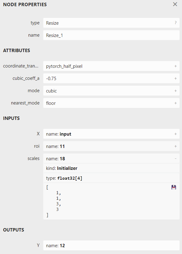
其中,展开 scales,可以看到 scales 是一个长度为 4 的一维张量,其内容为 [1, 1, 3, 3], 表示 Resize 操作每一个维度的缩放系数;其类型为 Initializer,表示这个值是根据常量直接初始化出来的。如果我们能够自己生成一个 ONNX 的 Resize 算子,让 scales 成为一个可变量而不是常量,就像它上面的 X 一样,那这个超分辨率模型就能动态缩放了。
现有实现插值的 PyTorch 算子有一套规定好的映射到 ONNX Resize 算子的方法,这些映射出的 Resize 算子的 scales 只能是常量,无法满足我们的需求。我们得自己定义一个实现插值的 PyTorch 算子,然后让它映射到一个我们期望的 ONNX Resize 算子上。
下面的脚本定义了一个 PyTorch 插值算子,并在模型里使用了它。我们先通过运行模型来验证该算子的正确性:
import torch
from torch import nn
from torch.nn.functional import interpolate
import torch.onnx
import cv2
import numpy as np


class NewInterpolate(torch.autograd.Function):

    @staticmethod
    def symbolic(g, input, scales):
        return g.op("Resize",
                    input,
                    g.op("Constant",
                         value_t=torch.tensor([], dtype=torch.float32)),
                    scales,
                    coordinate_transformation_mode_s="pytorch_half_pixel",
                    cubic_coeff_a_f=-0.75,
                    mode_s='cubic',
                    nearest_mode_s="floor")

    @staticmethod
    def forward(ctx, input, scales):
        scales = scales.tolist()[-2:]
        return interpolate(input,
                           scale_factor=scales,
                           mode='bicubic',
                           align_corners=False)


class StrangeSuperResolutionNet(nn.Module):

    def __init__(self):
        super().__init__()

        self.conv1 = nn.Conv2d(3, 64, kernel_size=9, padding=4)
        self.conv2 = nn.Conv2d(64, 32, kernel_size=1, padding=0)
        self.conv3 = nn.Conv2d(32, 3, kernel_size=5, padding=2)

        self.relu = nn.ReLU()

    def forward(self, x, upscale_factor):
        x = NewInterpolate.apply(x, upscale_factor)
        out = self.relu(self.conv1(x))
        out = self.relu(self.conv2(out))
        out = self.conv3(out)
        return out


def init_torch_model():
    torch_model = StrangeSuperResolutionNet()

    state_dict = torch.load('srcnn.pth')['state_dict']

    # Adapt the checkpoint
    for old_key in list(state_dict.keys()):
        new_key = '.'.join(old_key.split('.')[1:])
        state_dict[new_key] = state_dict.pop(old_key)

    torch_model.load_state_dict(state_dict)
    torch_model.eval()
    return torch_model


model = init_torch_model()
factor = torch.tensor([1, 1, 3, 3], dtype=torch.float)

input_img = cv2.imread('face.png').astype(np.float32)

# HWC to NCHW
input_img = np.transpose(input_img, [2, 0, 1])
input_img = np.expand_dims(input_img, 0)

# Inference
torch_output = model(torch.from_numpy(input_img), factor).detach().numpy()

# NCHW to HWC
torch_output = np.squeeze(torch_output, 0)
torch_output = np.clip(torch_output, 0, 255)
torch_output = np.transpose(torch_output, [1, 2, 0]).astype(np.uint8)

# Show image
cv2.imwrite("face_torch_3.png", torch_output)
模型运行正常的话,一幅放大3倍的超分辨率图片会保存在”face_torch_3.png”中,其内容和”face_torch.png”完全相同。
在刚刚那个脚本中,我们定义 PyTorch 插值算子的代码如下:
class NewInterpolate(torch.autograd.Function):

    @staticmethod
    def symbolic(g, input, scales):
        return g.op("Resize",
                    input,
                    g.op("Constant",
                         value_t=torch.tensor([], dtype=torch.float32)),
                    scales,
                    coordinate_transformation_mode_s="pytorch_half_pixel",
                    cubic_coeff_a_f=-0.75,
                    mode_s='cubic',
                    nearest_mode_s="floor")

    @staticmethod
    def forward(ctx, input, scales):
        scales = scales.tolist()[-2:]
        return interpolate(input,
                           scale_factor=scales,
                           mode='bicubic',
                           align_corners=False)
在具体介绍这个算子的实现前,让我们先理清一下思路。我们希望新的插值算子有两个输入,一个是被用于操作的图像,一个是图像的放缩比例。前面讲到,为了对接 ONNX 中 Resize 算子的 scales 参数,这个放缩比例是一个 [1, 1, x, x] 的张量,其中 x 为放大倍数。在之前放大3倍的模型中,这个参数被固定成了[1, 1, 3, 3]。因此,在插值算子中,我们希望模型的第二个输入是一个 [1, 1, w, h] 的张量,其中 w 和 h 分别是图片宽和高的放大倍数。
搞清楚了插值算子的输入,再看一看算子的具体实现。算子的推理行为由算子的 forward 方法决定。该方法的第一个参数必须为 ctx,后面的参数为算子的自定义输入,我们设置两个输入,分别为被操作的图像和放缩比例。为保证推理正确,需要把 [1, 1, w, h] 格式的输入对接到原来的 interpolate 函数上。我们的做法是截取输入张量的后两个元素,把这两个元素以 list 的格式传入 interpolate 的 scale_factor 参数。
接下来,我们要决定新算子映射到 ONNX 算子的方法。映射到 ONNX 的方法由一个算子的 symbolic 方法决定。symbolic 方法第一个参数必须是g,之后的参数是算子的自定义输入,和 forward 函数一样。ONNX 算子的具体定义由 g.op 实现。g.op 的每个参数都可以映射到 ONNX 中的算子属性:
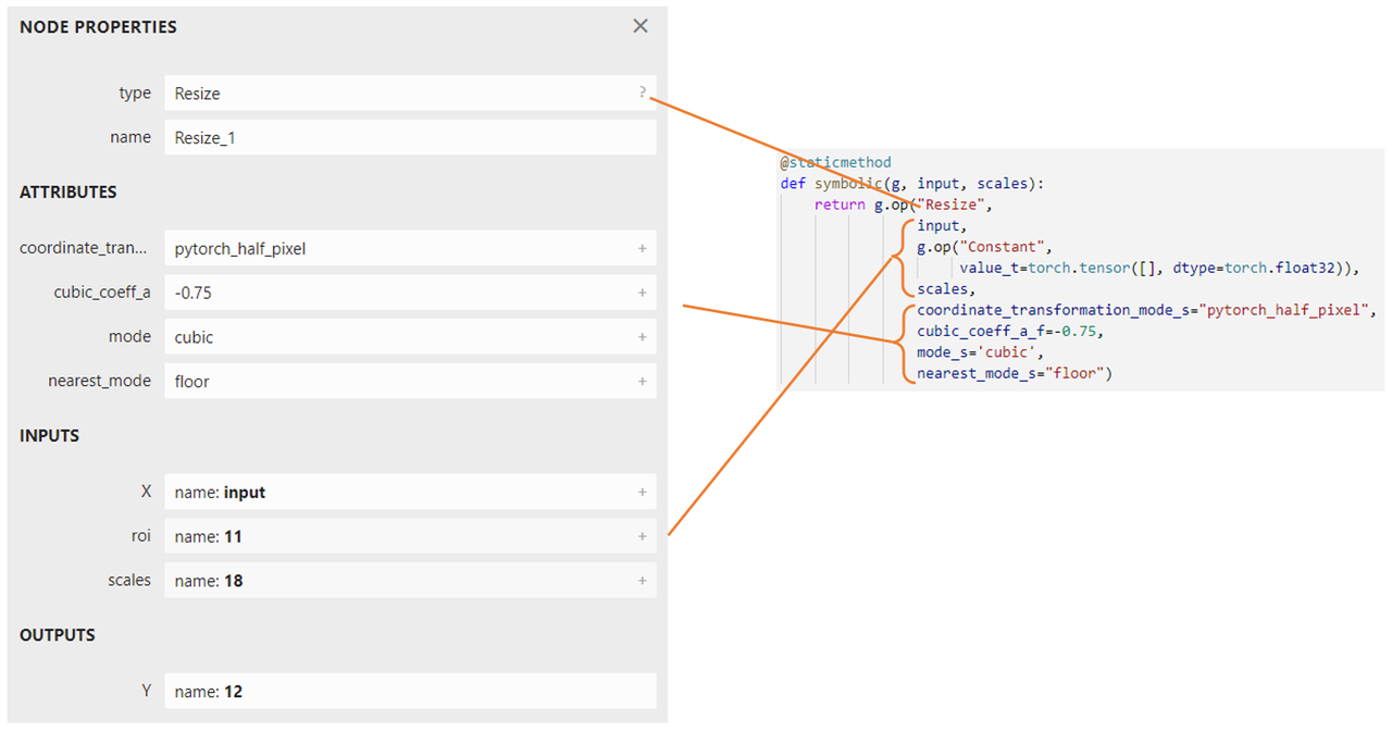
对于其他参数,我们可以照着现在的 Resize 算子填。而要注意的是,我们现在希望 scales 参数是由输入动态决定的。因此,在填入 ONNX 的 scales 时,我们要把 symbolic 方法的输入参数中的 scales 填入。
接着,让我们把新模型导出成 ONNX 模型:
x = torch.randn(1, 3, 256, 256)

with torch.no_grad():
    torch.onnx.export(model, (x, factor),
                      "srcnn3.onnx",
                      opset_version=11,
                      input_names=['input', 'factor'],
                      output_names=['output'])
把导出的 ” srcnn3.onnx ” 进行可视化:
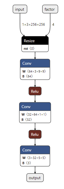
可以看到,正如我们所期望的,导出的 ONNX 模型有了两个输入!第二个输入表示图像的放缩比例。
之前在验证 PyTorch 模型和导出 ONNX 模型时,我们宽高的缩放比例设置成了 3x3。现在,在用 ONNX Runtime 推理时,我们尝试使用 4x4 的缩放比例:
import onnxruntime

input_factor = np.array([1, 1, 4, 4], dtype=np.float32)
ort_session = onnxruntime.InferenceSession("srcnn3.onnx")
ort_inputs = {'input': input_img, 'factor': input_factor}
ort_output = ort_session.run(None, ort_inputs)[0]

ort_output = np.squeeze(ort_output, 0)
ort_output = np.clip(ort_output, 0, 255)
ort_output = np.transpose(ort_output, [1, 2, 0]).astype(np.uint8)
cv2.imwrite("face_ort_3.png", ort_output)
运行上面的代码,可以得到一个边长放大4倍的超分辨率图片 “face_ort_3.png”。动态的超分辨率模型生成成功了!只要修改 input_factor,我们就可以自由地控制图片的缩放比例。
我们刚刚的工作,实际上是绕过 PyTorch 本身的限制,凭空“捏”出了一个 ONNX 算子。事实上,我们不仅可以创建现有的 ONNX 算子,还可以定义新的 ONNX 算子以拓展 ONNX 的表达能力。后续教程中我们将介绍自定义新 ONNX 算子的方法。
总结
通过学习前两篇教程,我们走完了整个部署流水线,成功部署了支持动态放大倍数的超分辨率模型。在这个过程中,我们既学会了如何简单地调用各框架的API实现模型部署,又学到了如何分析并尝试解决模型部署时碰到的难题。
同样,让我们总结一下本篇教程的知识点:
模型部署中常见的几类困难有:模型的动态化;新算子的实现;框架间的兼容。
PyTorch 转 ONNX,实际上就是把每一个操作转化成 ONNX 定义的某一个算子。比如对于 PyTorch 中的 Upsample 和 interpolate,在转 ONNX 后最终都会成为 ONNX 的 Resize 算子。
通过修改继承自 torch.autograd.Function 的算子的 symbolic 方法,可以改变该算子映射到 ONNX 算子的行为。
至此,”部署第一个模型“的教程算是告一段落了。是不是觉得学到的知识还不够多?没关系,在接下来的几篇教程中,我们将结合 MMDeploy ,重点介绍 ONNX 中间表示和 ONNX Runtime/TensorRT 推理引擎的知识,让大家学会如何部署更复杂的模型。